SIGGRAPH向来是Computer Graphics研究的风向标。今天粗略过了一遍SigGRAPH2009论文,乱弹一下心得:
1.hair modeling and simulation and rendering 主题真是耐做,有两篇都是关于此主题的:“Example-based hair geometry synthesis ”和“Detail preserving continuum simulation of straight hair ”。
2.”Fluid simulation“研究同样是常青树,专门有一个Session。
3.国内的强人“Kun Zhou“还是发了3篇论文。
4.最”牛气“的论文是”Semantic Deformation Transfer“,名字很短,正文只有6页,12篇参考文献;
5.有两个关于”Character animation”的session,8篇论文,占到总论文的10%;
6.有两个跟physics相关的session,“Physically based modeling: from contact to capture”和“Reduced physics for animation”,拓展一点,如果把“Creating natural variations”自然也看出跟物理相关的话,总共有三个session。物理是王道呀。
7. simulation方面,除了“Fluid simulation”session,还有“Directable, high-resolution simulation of fire on the GPU“,“Detail preserving continuum simulation of straight hair ”和“Interactive simulation of surgical needle insertion and steering ”。
2009-09-20


2009-09-13
Oops, I got it.
前天出了一个问题(http://leepyzh.blogspot.com/2009/09/cg-lighting.html),是在看Cg例子“09_vertex_lighting”的时候,为了计算光照,他有一个对modelview矩阵求逆的过程,这是由于GPU顶点程序的顶点位于model坐标系,将灯光和眼睛的位置逆变换到物体的位置空间,这样在同一空间里面可以求解。
看了这个例子后,总觉得求逆是一件费时的事,干吗不把顶点坐标和向量变换到世界坐标系?这样也可以在同一空间求解呀。但是修改程序后,感觉灯光的位置有些偏差,百思不得其解。Cg程序如下:
#if 1
//here is my code to change the vertex coord & normal to world space
float4 worldcoordinate = mul(modelToWorld, position);
float3 P = worldcoordinate.xyz;
float4 Normal4;
Normal4[0] = normal[0];
Normal4[1] = normal[1];
Normal4[2] = normal[2];
Normal4[3] = 1;
float4 N4 = mul(modelToWorld, Normal4);
float3 N = N4.xyz;
N = normalize(N);
#else
//here is the formal code
float3 P = position.xyz;
float3 N = normal;
#endif
今天,看到“18_cube_map_reflection”的时候发现他用到这个想法。呵呵,至少心里放心了。看看例子的代码,比我的简洁多了:
// Compute position and normal in world space
float3 P = mul(modelToWorld, position).xyz;
float3 N = mul((float3x3)modelToWorld, normal);
N = normalize(N);
经过盘查,我终于找到了问题所在,原来是向量相乘的时候出了问题:
Normal4[3] = 1;
其实对于向量来说,第四维是没有意义的。如果赋值为1,那么需要将原点看成起点,在两个变换完成后,然后相减得到新的向量。最简单的方法,将第四维赋值为0。从几何上可以这么理解:平移不改变向量。
到此,似乎问题已经解决。当接着往下看Cg tutorial时,又让我吃了一大惊,他说:
If the modeling transform scales positions nonuniformly, you must multiply normal by the inverse transpose of the modeling matrix ( modelToWorldInvTrans ), rather than simply by modelToWorld.
是呀。旋转和平移时,点的相对位置不会改变,所以直接变换向量没有问题;然后,不均匀的缩放时,平面发生变形,此时,法向不能简单地乘以变换矩阵而得到。
网上一位老兄给出了总结,我想应该是对的:
1.如果变换模型位置的仅仅是rotation 或 translation, 可以用该Matrix直接作用于法线,获得最终的法线.
2.如果传输模型的Matrix 是同比例scale, 用该matrix作用法线后,获得的新法线需要重新normalize
3.如果非同比例scale的matrix,必须用该matrix的inverse后,再transpose来作用于该法线。
4. 具体内容可参考: Real-Time Shader Programming 82-83页。
Finally, 看来“09_vertex_lighting”的求逆阵还是个最好的、不会出错的解决方法。
看了这个例子后,总觉得求逆是一件费时的事,干吗不把顶点坐标和向量变换到世界坐标系?这样也可以在同一空间求解呀。但是修改程序后,感觉灯光的位置有些偏差,百思不得其解。Cg程序如下:
#if 1
//here is my code to change the vertex coord & normal to world space
float4 worldcoordinate = mul(modelToWorld, position);
float3 P = worldcoordinate.xyz;
float4 Normal4;
Normal4[0] = normal[0];
Normal4[1] = normal[1];
Normal4[2] = normal[2];
Normal4[3] = 1;
float4 N4 = mul(modelToWorld, Normal4);
float3 N = N4.xyz;
N = normalize(N);
#else
//here is the formal code
float3 P = position.xyz;
float3 N = normal;
#endif
今天,看到“18_cube_map_reflection”的时候发现他用到这个想法。呵呵,至少心里放心了。看看例子的代码,比我的简洁多了:
// Compute position and normal in world space
float3 P = mul(modelToWorld, position).xyz;
float3 N = mul((float3x3)modelToWorld, normal);
N = normalize(N);
经过盘查,我终于找到了问题所在,原来是向量相乘的时候出了问题:
Normal4[3] = 1;
其实对于向量来说,第四维是没有意义的。如果赋值为1,那么需要将原点看成起点,在两个变换完成后,然后相减得到新的向量。最简单的方法,将第四维赋值为0。从几何上可以这么理解:平移不改变向量。
到此,似乎问题已经解决。当接着往下看Cg tutorial时,又让我吃了一大惊,他说:
If the modeling transform scales positions nonuniformly, you must multiply normal by the inverse transpose of the modeling matrix ( modelToWorldInvTrans ), rather than simply by modelToWorld.
是呀。旋转和平移时,点的相对位置不会改变,所以直接变换向量没有问题;然后,不均匀的缩放时,平面发生变形,此时,法向不能简单地乘以变换矩阵而得到。
网上一位老兄给出了总结,我想应该是对的:
1.如果变换模型位置的仅仅是rotation 或 translation, 可以用该Matrix直接作用于法线,获得最终的法线.
2.如果传输模型的Matrix 是同比例scale, 用该matrix作用法线后,获得的新法线需要重新normalize
3.如果非同比例scale的matrix,必须用该matrix的inverse后,再transpose来作用于该法线。
4. 具体内容可参考: Real-Time Shader Programming 82-83页。
Finally, 看来“09_vertex_lighting”的求逆阵还是个最好的、不会出错的解决方法。
2009-09-12
Cg Vertex prgram & fragment program.

顶点程序输入:
1.未经过任何变换的顶点,坐标和法向为均为物体空间,不是世界坐标系;
2. 纹理坐标;
3. 顶点被(OpenGL程序)设置的颜色。
顶点程序输出:
1. 变换到投影坐标系的顶点坐标【必须】;
2. 纹理坐标【可选,或者是顶点程序要传给片段程序的参数,封装在纹理坐标里】;
3. 顶点光照后的颜色【可选,也可在fragment程序中完成】;
片段程序的输入:
1.顶点经过二次线性插值后的片段的颜色【可选】;
2.纹理坐标【可选】;
片段程序的输出:
1. 片段颜色【必须,纹理映射后的颜色或者按片段进行“精确”光照后的颜色或者直接pass through】。
2009-09-11
Cg Lighting......
今天看到Cg中OpenGL的例子“09_vertex_lighting”,例子简洁明了,用生动地展示了基本光照过程。真是爱死Cg了,“The Cg Tutorial"这本书的作者真是太牛了。
light.......
{
float3 P = position.xyz; //current point
float3 N = normal;
// Compute emissive term
float3 emissive = Ke;
// Compute ambient term
float3 ambient = Ka * globalAmbient;
// Compute the diffuse term
float3 L = normalize(lightPosition - P);
float diffuseLight = max(dot(N, L), 0);
float3 diffuse = Kd * lightColor * diffuseLight;
// Compute the specular term
float3 V = normalize(eyePosition - P);
float3 H = normalize(L + V);
float specularLight = pow(max(dot(N, H), 0), shininess);
if (diffuseLight <= 0) specularLight = 0;
float3 specular = Ks * lightColor * specularLight;
color.xyz = emissive + ambient + diffuse + specular;
color.w = 1;
}
几点理解:
1)emissive并不是场景中的光源,它不能照亮其他物体,而自身将会呈现一种单一的颜色;
2)镜面反射取出眼睛和灯光中间向量,与法向求夹角。shininess = 0,光晕最大;shininess增加,呈指数衰减,最后shininess->∽时,只有dot(N, H)=1也就是N和H重合时,采用光斑;
3)在GPU的顶点程序中,传进来的顶点position是未经过任何变换的坐标值,它处于模型坐标系中;而眼睛和光源的位置是在世界坐标系中定义的。所以,GPU计算光照时,必须将眼睛和光源的坐标进行反推到模型坐标系,具体是对modelMatrix求逆,在乘上眼睛和光源的坐标向量;
4)我尝试将modelMatrix传入顶点程序,以将position和normal转入世界坐标系求光照,但是得到错误的结果,思考中......
5)本例子提供了求矩阵逆的函数,弓虽!
/* Invert a row-major (C-style) 4x4 matrix. */
static void invertMatrix(float *out, const float *m)
{
/* Assumes matrices are ROW major. */
#define SWAP_ROWS(a, b) { GLdouble *_tmp = a; (a)=(b); (b)=_tmp; }
#define MAT(m,r,c) (m)[(r)*4+(c)]
double wtmp[4][8];
double m0, m1, m2, m3, s;
double *r0, *r1, *r2, *r3;
r0 = wtmp[0], r1 = wtmp[1], r2 = wtmp[2], r3 = wtmp[3];
r0[0] = MAT(m,0,0), r0[1] = MAT(m,0,1),
r0[2] = MAT(m,0,2), r0[3] = MAT(m,0,3),
r0[4] = 1.0, r0[5] = r0[6] = r0[7] = 0.0,
r1[0] = MAT(m,1,0), r1[1] = MAT(m,1,1),
r1[2] = MAT(m,1,2), r1[3] = MAT(m,1,3),
r1[5] = 1.0, r1[4] = r1[6] = r1[7] = 0.0,
r2[0] = MAT(m,2,0), r2[1] = MAT(m,2,1),
r2[2] = MAT(m,2,2), r2[3] = MAT(m,2,3),
r2[6] = 1.0, r2[4] = r2[5] = r2[7] = 0.0,
r3[0] = MAT(m,3,0), r3[1] = MAT(m,3,1),
r3[2] = MAT(m,3,2), r3[3] = MAT(m,3,3),
r3[7] = 1.0, r3[4] = r3[5] = r3[6] = 0.0;
/* Choose myPivot, or die. */
if (fabs(r3[0])>fabs(r2[0])) SWAP_ROWS(r3, r2);
if (fabs(r2[0])>fabs(r1[0])) SWAP_ROWS(r2, r1);
if (fabs(r1[0])>fabs(r0[0])) SWAP_ROWS(r1, r0);
if (0.0 == r0[0]) {
assert(!"could not invert matrix");
}
/* Eliminate first variable. */
m1 = r1[0]/r0[0]; m2 = r2[0]/r0[0]; m3 = r3[0]/r0[0];
s = r0[1]; r1[1] -= m1 * s; r2[1] -= m2 * s; r3[1] -= m3 * s;
s = r0[2]; r1[2] -= m1 * s; r2[2] -= m2 * s; r3[2] -= m3 * s;
s = r0[3]; r1[3] -= m1 * s; r2[3] -= m2 * s; r3[3] -= m3 * s;
s = r0[4];
if (s != 0.0) { r1[4] -= m1 * s; r2[4] -= m2 * s; r3[4] -= m3 * s; }
s = r0[5];
if (s != 0.0) { r1[5] -= m1 * s; r2[5] -= m2 * s; r3[5] -= m3 * s; }
s = r0[6];
if (s != 0.0) { r1[6] -= m1 * s; r2[6] -= m2 * s; r3[6] -= m3 * s; }
s = r0[7];
if (s != 0.0) { r1[7] -= m1 * s; r2[7] -= m2 * s; r3[7] -= m3 * s; }
/* Choose myPivot, or die. */
if (fabs(r3[1])>fabs(r2[1])) SWAP_ROWS(r3, r2);
if (fabs(r2[1])>fabs(r1[1])) SWAP_ROWS(r2, r1);
if (0.0 == r1[1]) {
assert(!"could not invert matrix");
}
/* Eliminate second variable. */
m2 = r2[1]/r1[1]; m3 = r3[1]/r1[1];
r2[2] -= m2 * r1[2]; r3[2] -= m3 * r1[2];
r2[3] -= m2 * r1[3]; r3[3] -= m3 * r1[3];
s = r1[4]; if (0.0 != s) { r2[4] -= m2 * s; r3[4] -= m3 * s; }
s = r1[5]; if (0.0 != s) { r2[5] -= m2 * s; r3[5] -= m3 * s; }
s = r1[6]; if (0.0 != s) { r2[6] -= m2 * s; r3[6] -= m3 * s; }
s = r1[7]; if (0.0 != s) { r2[7] -= m2 * s; r3[7] -= m3 * s; }
/* Choose myPivot, or die. */
if (fabs(r3[2])>fabs(r2[2])) SWAP_ROWS(r3, r2);
if (0.0 == r2[2]) {
assert(!"could not invert matrix");
}
/* Eliminate third variable. */
m3 = r3[2]/r2[2];
r3[3] -= m3 * r2[3], r3[4] -= m3 * r2[4],
r3[5] -= m3 * r2[5], r3[6] -= m3 * r2[6],
r3[7] -= m3 * r2[7];
/* Last check. */
if (0.0 == r3[3]) {
assert(!"could not invert matrix");
}
s = 1.0/r3[3]; /* Now back substitute row 3. */
r3[4] *= s; r3[5] *= s; r3[6] *= s; r3[7] *= s;
m2 = r2[3]; /* Now back substitute row 2. */
s = 1.0/r2[2];
r2[4] = s * (r2[4] - r3[4] * m2), r2[5] = s * (r2[5] - r3[5] * m2),
r2[6] = s * (r2[6] - r3[6] * m2), r2[7] = s * (r2[7] - r3[7] * m2);
m1 = r1[3];
r1[4] -= r3[4] * m1, r1[5] -= r3[5] * m1,
r1[6] -= r3[6] * m1, r1[7] -= r3[7] * m1;
m0 = r0[3];
r0[4] -= r3[4] * m0, r0[5] -= r3[5] * m0,
r0[6] -= r3[6] * m0, r0[7] -= r3[7] * m0;
m1 = r1[2]; /* Now back substitute row 1. */
s = 1.0/r1[1];
r1[4] = s * (r1[4] - r2[4] * m1), r1[5] = s * (r1[5] - r2[5] * m1),
r1[6] = s * (r1[6] - r2[6] * m1), r1[7] = s * (r1[7] - r2[7] * m1);
m0 = r0[2];
r0[4] -= r2[4] * m0, r0[5] -= r2[5] * m0,
r0[6] -= r2[6] * m0, r0[7] -= r2[7] * m0;
m0 = r0[1]; /* Now back substitute row 0. */
s = 1.0/r0[0];
r0[4] = s * (r0[4] - r1[4] * m0), r0[5] = s * (r0[5] - r1[5] * m0),
r0[6] = s * (r0[6] - r1[6] * m0), r0[7] = s * (r0[7] - r1[7] * m0);
MAT(out,0,0) = r0[4]; MAT(out,0,1) = r0[5],
MAT(out,0,2) = r0[6]; MAT(out,0,3) = r0[7],
MAT(out,1,0) = r1[4]; MAT(out,1,1) = r1[5],
MAT(out,1,2) = r1[6]; MAT(out,1,3) = r1[7],
MAT(out,2,0) = r2[4]; MAT(out,2,1) = r2[5],
MAT(out,2,2) = r2[6]; MAT(out,2,3) = r2[7],
MAT(out,3,0) = r3[4]; MAT(out,3,1) = r3[5],
MAT(out,3,2) = r3[6]; MAT(out,3,3) = r3[7];
#undef MAT
#undef SWAP_ROWS
}
light.......
{
float3 P = position.xyz; //current point
float3 N = normal;
// Compute emissive term
float3 emissive = Ke;
// Compute ambient term
float3 ambient = Ka * globalAmbient;
// Compute the diffuse term
float3 L = normalize(lightPosition - P);
float diffuseLight = max(dot(N, L), 0);
float3 diffuse = Kd * lightColor * diffuseLight;
// Compute the specular term
float3 V = normalize(eyePosition - P);
float3 H = normalize(L + V);
float specularLight = pow(max(dot(N, H), 0), shininess);
if (diffuseLight <= 0) specularLight = 0;
float3 specular = Ks * lightColor * specularLight;
color.xyz = emissive + ambient + diffuse + specular;
color.w = 1;
}
几点理解:
1)emissive并不是场景中的光源,它不能照亮其他物体,而自身将会呈现一种单一的颜色;
2)镜面反射取出眼睛和灯光中间向量,与法向求夹角。shininess = 0,光晕最大;shininess增加,呈指数衰减,最后shininess->∽时,只有dot(N, H)=1也就是N和H重合时,采用光斑;
3)在GPU的顶点程序中,传进来的顶点position是未经过任何变换的坐标值,它处于模型坐标系中;而眼睛和光源的位置是在世界坐标系中定义的。所以,GPU计算光照时,必须将眼睛和光源的坐标进行反推到模型坐标系,具体是对modelMatrix求逆,在乘上眼睛和光源的坐标向量;
4)我尝试将modelMatrix传入顶点程序,以将position和normal转入世界坐标系求光照,但是得到错误的结果,思考中......
5)本例子提供了求矩阵逆的函数,弓虽!
/* Invert a row-major (C-style) 4x4 matrix. */
static void invertMatrix(float *out, const float *m)
{
/* Assumes matrices are ROW major. */
#define SWAP_ROWS(a, b) { GLdouble *_tmp = a; (a)=(b); (b)=_tmp; }
#define MAT(m,r,c) (m)[(r)*4+(c)]
double wtmp[4][8];
double m0, m1, m2, m3, s;
double *r0, *r1, *r2, *r3;
r0 = wtmp[0], r1 = wtmp[1], r2 = wtmp[2], r3 = wtmp[3];
r0[0] = MAT(m,0,0), r0[1] = MAT(m,0,1),
r0[2] = MAT(m,0,2), r0[3] = MAT(m,0,3),
r0[4] = 1.0, r0[5] = r0[6] = r0[7] = 0.0,
r1[0] = MAT(m,1,0), r1[1] = MAT(m,1,1),
r1[2] = MAT(m,1,2), r1[3] = MAT(m,1,3),
r1[5] = 1.0, r1[4] = r1[6] = r1[7] = 0.0,
r2[0] = MAT(m,2,0), r2[1] = MAT(m,2,1),
r2[2] = MAT(m,2,2), r2[3] = MAT(m,2,3),
r2[6] = 1.0, r2[4] = r2[5] = r2[7] = 0.0,
r3[0] = MAT(m,3,0), r3[1] = MAT(m,3,1),
r3[2] = MAT(m,3,2), r3[3] = MAT(m,3,3),
r3[7] = 1.0, r3[4] = r3[5] = r3[6] = 0.0;
/* Choose myPivot, or die. */
if (fabs(r3[0])>fabs(r2[0])) SWAP_ROWS(r3, r2);
if (fabs(r2[0])>fabs(r1[0])) SWAP_ROWS(r2, r1);
if (fabs(r1[0])>fabs(r0[0])) SWAP_ROWS(r1, r0);
if (0.0 == r0[0]) {
assert(!"could not invert matrix");
}
/* Eliminate first variable. */
m1 = r1[0]/r0[0]; m2 = r2[0]/r0[0]; m3 = r3[0]/r0[0];
s = r0[1]; r1[1] -= m1 * s; r2[1] -= m2 * s; r3[1] -= m3 * s;
s = r0[2]; r1[2] -= m1 * s; r2[2] -= m2 * s; r3[2] -= m3 * s;
s = r0[3]; r1[3] -= m1 * s; r2[3] -= m2 * s; r3[3] -= m3 * s;
s = r0[4];
if (s != 0.0) { r1[4] -= m1 * s; r2[4] -= m2 * s; r3[4] -= m3 * s; }
s = r0[5];
if (s != 0.0) { r1[5] -= m1 * s; r2[5] -= m2 * s; r3[5] -= m3 * s; }
s = r0[6];
if (s != 0.0) { r1[6] -= m1 * s; r2[6] -= m2 * s; r3[6] -= m3 * s; }
s = r0[7];
if (s != 0.0) { r1[7] -= m1 * s; r2[7] -= m2 * s; r3[7] -= m3 * s; }
/* Choose myPivot, or die. */
if (fabs(r3[1])>fabs(r2[1])) SWAP_ROWS(r3, r2);
if (fabs(r2[1])>fabs(r1[1])) SWAP_ROWS(r2, r1);
if (0.0 == r1[1]) {
assert(!"could not invert matrix");
}
/* Eliminate second variable. */
m2 = r2[1]/r1[1]; m3 = r3[1]/r1[1];
r2[2] -= m2 * r1[2]; r3[2] -= m3 * r1[2];
r2[3] -= m2 * r1[3]; r3[3] -= m3 * r1[3];
s = r1[4]; if (0.0 != s) { r2[4] -= m2 * s; r3[4] -= m3 * s; }
s = r1[5]; if (0.0 != s) { r2[5] -= m2 * s; r3[5] -= m3 * s; }
s = r1[6]; if (0.0 != s) { r2[6] -= m2 * s; r3[6] -= m3 * s; }
s = r1[7]; if (0.0 != s) { r2[7] -= m2 * s; r3[7] -= m3 * s; }
/* Choose myPivot, or die. */
if (fabs(r3[2])>fabs(r2[2])) SWAP_ROWS(r3, r2);
if (0.0 == r2[2]) {
assert(!"could not invert matrix");
}
/* Eliminate third variable. */
m3 = r3[2]/r2[2];
r3[3] -= m3 * r2[3], r3[4] -= m3 * r2[4],
r3[5] -= m3 * r2[5], r3[6] -= m3 * r2[6],
r3[7] -= m3 * r2[7];
/* Last check. */
if (0.0 == r3[3]) {
assert(!"could not invert matrix");
}
s = 1.0/r3[3]; /* Now back substitute row 3. */
r3[4] *= s; r3[5] *= s; r3[6] *= s; r3[7] *= s;
m2 = r2[3]; /* Now back substitute row 2. */
s = 1.0/r2[2];
r2[4] = s * (r2[4] - r3[4] * m2), r2[5] = s * (r2[5] - r3[5] * m2),
r2[6] = s * (r2[6] - r3[6] * m2), r2[7] = s * (r2[7] - r3[7] * m2);
m1 = r1[3];
r1[4] -= r3[4] * m1, r1[5] -= r3[5] * m1,
r1[6] -= r3[6] * m1, r1[7] -= r3[7] * m1;
m0 = r0[3];
r0[4] -= r3[4] * m0, r0[5] -= r3[5] * m0,
r0[6] -= r3[6] * m0, r0[7] -= r3[7] * m0;
m1 = r1[2]; /* Now back substitute row 1. */
s = 1.0/r1[1];
r1[4] = s * (r1[4] - r2[4] * m1), r1[5] = s * (r1[5] - r2[5] * m1),
r1[6] = s * (r1[6] - r2[6] * m1), r1[7] = s * (r1[7] - r2[7] * m1);
m0 = r0[2];
r0[4] -= r2[4] * m0, r0[5] -= r2[5] * m0,
r0[6] -= r2[6] * m0, r0[7] -= r2[7] * m0;
m0 = r0[1]; /* Now back substitute row 0. */
s = 1.0/r0[0];
r0[4] = s * (r0[4] - r1[4] * m0), r0[5] = s * (r0[5] - r1[5] * m0),
r0[6] = s * (r0[6] - r1[6] * m0), r0[7] = s * (r0[7] - r1[7] * m0);
MAT(out,0,0) = r0[4]; MAT(out,0,1) = r0[5],
MAT(out,0,2) = r0[6]; MAT(out,0,3) = r0[7],
MAT(out,1,0) = r1[4]; MAT(out,1,1) = r1[5],
MAT(out,1,2) = r1[6]; MAT(out,1,3) = r1[7],
MAT(out,2,0) = r2[4]; MAT(out,2,1) = r2[5],
MAT(out,2,2) = r2[6]; MAT(out,2,3) = r2[7],
MAT(out,3,0) = r3[4]; MAT(out,3,1) = r3[5],
MAT(out,3,2) = r3[6]; MAT(out,3,3) = r3[7];
#undef MAT
#undef SWAP_ROWS
}
2009-09-10
Z Buffer or Depth Buffer.
在投影空间中,z的范围是[-1,+1]。在OpenGL中,默认情况下,最接近眼睛的片断(在近截面上)被映射到0.0,离眼睛最远的片断(在远截面上)映射到1.0。这个映射调整应该是线性的(没有查到正式文献)。当然,还可用glDepthRange调节深度值范围。
在正交投影中距离和Z值的关系是线性的,但在透视投影中却不是的。在透视投影中,情况发生了变化,还是看看映射公式:
z'= f(z)/w' = (Zfar+Znear) / ( Zfar – Znear ) + [2* Zfar*Znear / ( Zfar – Znear )]/z
这个映射是个双曲线:

下面来理解(http://www.cppblog.com/zmj/archive/2008/03/14/14122.html)给出的这几句话:
1. 在透视投影中这种关系是非线性的,而且非线性的程度与Frustum函数中的far/near(或gluPerspective函数中的zFar/zNear)成比例——也不是严格成比例,因为有一个Zfar*Znear 在。
2. 这种非线性在靠近近截面时增加了Z值的精度,而且增加了深度缓存的效率;但是在视见体的其它部分则降低了精度,也就减少了深度缓存的精确性——在上图,将[-Zfar,-Znear]之间等分,呵呵,靠近-Znear得到的Z’的范围显然大得多。
3. 根据经验,far/near比值大于1000会有这种不好的效果。所以一般far/near比值应小于1000。要想解决这个问题,最简单的方法是通过将近截面远离眼睛来降低far/near比值,其唯一的副作用是离眼睛很近的物体可能会被裁减掉,但在特定的应用程序中这很少是个问题,近截面的位置对X、Y坐标的投影没有影响,因此这对图像的影响很小——这个要牢记,呵呵。
2009-09-09
Inside CG transformation (III).
最后看一下投影矩阵,这是最复杂的一个变换。我们只看透视投影矩阵,平行投影会简单很多。
在前面Cg Studying(http://leepyzh.blogspot.com/2009/09/cg-studying.html)一文中,我们已经看到了透视投影变换的过程:将平头视锥体变换了边长为2,中心在原点的立方体,以便于后面的裁剪和消隐工作。过程如下:
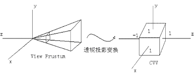 下面将变换设定在常用的情况上,就是投影平面的中心和xy平面的中心重合,即在上面右图的Z轴上。OpenGL中构建投影矩阵的函数是gluPerspective,其原型是:

static void buildPerspectiveMatrix(double fieldOfView,
double aspectRatio,
double zNear, double zFar,
float m[16])
{
double sine, cotangent, deltaZ;
double radians = fieldOfView / 2.0 * myPi / 180.0;
deltaZ = zFar - zNear;
sine = sin(radians);
/* Should be non-zero to avoid division by zero. */
assert(deltaZ);
assert(sine);
assert(aspectRatio);
cotangent = cos(radians) / sine;
m[0*4+0] = cotangent / aspectRatio;
m[0*4+1] = 0.0;
m[0*4+2] = 0.0;
m[0*4+3] = 0.0;
m[1*4+0] = 0.0;
m[1*4+1] = cotangent;
m[1*4+2] = 0.0;
m[1*4+3] = 0.0;
m[2*4+0] = 0.0;
m[2*4+1] = 0.0;
m[2*4+2] = -(zFar + zNear) / deltaZ;
m[2*4+3] = -2 * zNear * zFar / deltaZ;
m[3*4+0] = 0.0;
m[3*4+1] = 0.0;
m[3*4+2] = -1;
m[3*4+3] = 0;
}
至此,几个矩阵都推导完成了。
题外话:其实网上有很介绍矩阵的推导过程,包括很多教材上也有。但要真正理解,只有一种方法:实践出真知,自己动手。
Reference:
1. http://game.chinaitlab.com/arithmetic/28004.html;
2.http://blog.csdn.net/popy007/archive/2007/09/23/1797121.aspx;
3.http://blog.csdn.net/popy007/archive/2009/04/19/4091967.aspx。
在前面Cg Studying(http://leepyzh.blogspot.com/2009/09/cg-studying.html)一文中,我们已经看到了透视投影变换的过程:将平头视锥体变换了边长为2,中心在原点的立方体,以便于后面的裁剪和消隐工作。过程如下:
下面将变换设定在常用的情况上,就是投影平面的中心和xy平面的中心重合,即在上面右图的Z轴上。OpenGL中构建投影矩阵的函数是gluPerspective,其原型是: void gluPerspective(
GLdouble fovy, //角度
GLdouble aspect,//视景体的宽高比
GLdouble zNear,//沿z轴方向的两裁面之间的距离的近处
GLdouble zFar //沿z轴方向的两裁面之间的距离的远处
)
考虑上边界情况,对于眼坐标系来说:y=-ztan(fovy/2), 而对于投影坐标系来说:y'=1.
很显然,y的映射为:y'=-y/(ztan(fovy/2)=-ycot(fovy/2)/z。 考虑z相同的情况,此时y‘是y的单调增函数(考虑y>0情况)。所以这个映射也符合视锥内部的点。
对于y的负边界来说,情况类似。对于x来说,只需额外除以aspect这个值即可,因为:
aspect = width/height = x宽度/y高度
所以:x' = -xcot(fovy/2)/z/aspect.
由于这是非线性变换,要解决除以z,可以借助齐次坐标w来进行。令w'=-z,于是:
x' = xcot(fovy/2)/aspect.
y' = ycot(fovy/2)
w'=-z
那么z呢?其实在屏幕上显示后,z值对于颜色没有任何贡献。但是,消隐少不了z值,也就是所谓的z缓冲。对于z变换来说,一定要保留两个点的z值大小顺序不变,另外,为了归一化处理,将其映射到[-1,1]之间。而最后我们还可以在OpenGL中用glDepthRange调节深度值,这一点说明从这里算出来的Z值到最终的深度值之间还会有一个映射调整。好,话说远了,回来看看z的变换。
那么所需的Z变换有以下约束:
1)z=-znear--->z'=-1;
2)z=-zfar---->z'=+1;
3)映射具有单调减性质(因为有负号,所以单调减)
4)最终z'还要除以w'=-z
根据以上条件,构造映射:
f(z) = -z*(Zfar+Znear) / ( Zfar – Znear ) – 2* Zfar*Znear / ( Zfar – Znear )
z'= f(z)/w' = (Zfar+Znear) / ( Zfar – Znear ) + [2* Zfar*Znear / ( Zfar – Znear )]/z
验证一下,上述几个条件都满足。你要是想正向推导这个公式,也是可以的。可以参考后面的文献。
还是直接给出代码,一看就清楚:
static const double myPi = 3.14159265358979323846;static void buildPerspectiveMatrix(double fieldOfView,
double aspectRatio,
double zNear, double zFar,
float m[16])
{
double sine, cotangent, deltaZ;
double radians = fieldOfView / 2.0 * myPi / 180.0;
deltaZ = zFar - zNear;
sine = sin(radians);
/* Should be non-zero to avoid division by zero. */
assert(deltaZ);
assert(sine);
assert(aspectRatio);
cotangent = cos(radians) / sine;
m[0*4+0] = cotangent / aspectRatio;
m[0*4+1] = 0.0;
m[0*4+2] = 0.0;
m[0*4+3] = 0.0;
m[1*4+0] = 0.0;
m[1*4+1] = cotangent;
m[1*4+2] = 0.0;
m[1*4+3] = 0.0;
m[2*4+0] = 0.0;
m[2*4+1] = 0.0;
m[2*4+2] = -(zFar + zNear) / deltaZ;
m[2*4+3] = -2 * zNear * zFar / deltaZ;
m[3*4+0] = 0.0;
m[3*4+1] = 0.0;
m[3*4+2] = -1;
m[3*4+3] = 0;
}
至此,几个矩阵都推导完成了。
题外话:其实网上有很介绍矩阵的推导过程,包括很多教材上也有。但要真正理解,只有一种方法:实践出真知,自己动手。
Reference:
1. http://game.chinaitlab.com/arithmetic/28004.html;
2.http://blog.csdn.net/popy007/archive/2007/09/23/1797121.aspx;
3.http://blog.csdn.net/popy007/archive/2009/04/19/4091967.aspx。
2009-09-07
Inside CG transformation (II).
上一篇先解决了CG中的第一步变换,接下来来看viewMatrix。
视图变换实际上是坐标系的变换,将世界坐标系变换到眼坐标系(view ),这样做可以方便后面的投影(Projection)操作,因为投影是在眼坐标系中进行的。
建立眼坐标系用gluLookAt函数来实现,我们看看函数原型:
gluLookAt(double eyex, double eyey, double eyez, double centerx, double centery, double centerz, double upx, double upy, double upz)
这些参数中包括三种信息:眼睛的位置eye,视点中心位置center和向上的向量up。注意up不是y轴,只是指明了y轴的大致方向。
设眼睛的位置为原点,向量(eye-center)所得的向量为Z轴,y叉乘z得到x轴,再由x轴和z轴叉乘,反算出y轴。这就是眼坐标系的三个方向,设其单位向量为u、v、n。
然后就是坐标系之间的变换,这一点可以通过两种思路来完成:
1. 将眼坐标系变换到同世界坐标系重合。
2.代数的方法。
对于1而言,又有两种思路:
1. 代数上已经证明的公式:先移动eye的位置到世界坐标系的原点,再进行正交变换;
2. 由基本的变换合成,如下:
1)移动眼睛的位置到世界坐标系原点;
2)将眼坐标系绕世界坐标系x轴旋转,使得眼坐标系的z轴位于世界坐标系xoz平面;
3)将眼坐标系绕世界坐标系y轴旋转,使得眼坐标系的z轴和世界坐标系z轴重合;
4)将眼坐标系绕世界坐标系z轴旋转,使得眼坐标系的x、y轴和世界坐标系x、y轴重合;
这个步骤也需要很多的草稿纸,O(∩_∩)O
对于2,代数的方法,显得更简洁一些,看下图:
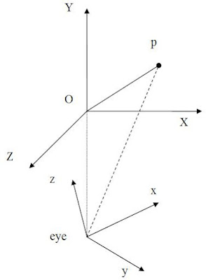
图中,对于任意的P点,向量减OP-Oeye= eyeP。再考虑eyeP向量,将其对眼坐标系的x/y/z轴进行投影,呵呵,就能得到P点在新坐标系中的坐标。投影很简单,用点乘即可。
于是,对于P点的新坐标P'(x',y',z'):
x' =(OP-Oeye).u = OP.u - Oeye.u =(x,y,z).(u[0],u[1],u[2]) -Oeye.(u[0],u[1],u[2]);
其中,u为眼坐标x轴方向的单位向量, x为P点的x坐标,u[0]为u向量的x值;其他类似。
y、z类似,我想你应该能写出矩阵来了吧,此处矩阵略过,直接看代码吧。
/* Build a row-major (C-style) 4x4 matrix transform based on the parameters for gluLookAt. */
static void buildLookAtMatrix(double eyex, double eyey, double eyez,
double centerx, double centery, double centerz,
double upx, double upy, double upz,float m[16])
{
double x[3], y[3], z[3], mag;
/* Difference eye and center vectors to make Z vector. */
z[0] = eyex - centerx;
z[1] = eyey - centery;
z[2] = eyez - centerz;
/* Normalize Z. */
mag = sqrt(z[0]*z[0] + z[1]*z[1] + z[2]*z[2]);
if (mag) {
z[0] /= mag;
z[1] /= mag;
z[2] /= mag;
}
/* Up vector makes Y vector. */
y[0] = upx;
y[1] = upy;
y[2] = upz;
/* X vector = Y cross Z. */
x[0] = y[1]*z[2] - y[2]*z[1];
x[1] = -y[0]*z[2] + y[2]*z[0];
x[2] = y[0]*z[1] - y[1]*z[0];
/* Recompute Y = Z cross X. */
y[0] = z[1]*x[2] - z[2]*x[1];
y[1] = -z[0]*x[2] + z[2]*x[0];
y[2] = z[0]*x[1] - z[1]*x[0];
/* Normalize X. */
mag = sqrt(x[0]*x[0] + x[1]*x[1] + x[2]*x[2]);
if (mag) {
x[0] /= mag;
x[1] /= mag;
x[2] /= mag;
}
/* Normalize Y. */
mag = sqrt(y[0]*y[0] + y[1]*y[1] + y[2]*y[2]);
if (mag) {
y[0] /= mag;
y[1] /= mag;
y[2] /= mag;
}
/* Build resulting view matrix. */
m[0*4+0] = x[0]; m[0*4+1] = x[1];
m[0*4+2] = x[2]; m[0*4+3] = -x[0]*eyex + -x[1]*eyey + -x[2]*eyez;
m[1*4+0] = y[0]; m[1*4+1] = y[1];
m[1*4+2] = y[2]; m[1*4+3] = -y[0]*eyex + -y[1]*eyey + -y[2]*eyez;
m[2*4+0] = z[0]; m[2*4+1] = z[1];
m[2*4+2] = z[2]; m[2*4+3] = -z[0]*eyex + -z[1]*eyey + -z[2]*eyez;
m[3*4+0] = 0.0; m[3*4+1] = 0.0; m[3*4+2] = 0.0; m[3*4+3] = 1.0;
}
到此,view矩阵已经OK了。
视图变换实际上是坐标系的变换,将世界坐标系变换到眼坐标系(view ),这样做可以方便后面的投影(Projection)操作,因为投影是在眼坐标系中进行的。
建立眼坐标系用gluLookAt函数来实现,我们看看函数原型:
gluLookAt(double eyex, double eyey, double eyez, double centerx, double centery, double centerz, double upx, double upy, double upz)
这些参数中包括三种信息:眼睛的位置eye,视点中心位置center和向上的向量up。注意up不是y轴,只是指明了y轴的大致方向。
设眼睛的位置为原点,向量(eye-center)所得的向量为Z轴,y叉乘z得到x轴,再由x轴和z轴叉乘,反算出y轴。这就是眼坐标系的三个方向,设其单位向量为u、v、n。
然后就是坐标系之间的变换,这一点可以通过两种思路来完成:
1. 将眼坐标系变换到同世界坐标系重合。
2.代数的方法。
对于1而言,又有两种思路:
1. 代数上已经证明的公式:先移动eye的位置到世界坐标系的原点,再进行正交变换;
2. 由基本的变换合成,如下:
1)移动眼睛的位置到世界坐标系原点;
2)将眼坐标系绕世界坐标系x轴旋转,使得眼坐标系的z轴位于世界坐标系xoz平面;
3)将眼坐标系绕世界坐标系y轴旋转,使得眼坐标系的z轴和世界坐标系z轴重合;
4)将眼坐标系绕世界坐标系z轴旋转,使得眼坐标系的x、y轴和世界坐标系x、y轴重合;
这个步骤也需要很多的草稿纸,O(∩_∩)O
对于2,代数的方法,显得更简洁一些,看下图:
图中,对于任意的P点,向量减OP-Oeye= eyeP。再考虑eyeP向量,将其对眼坐标系的x/y/z轴进行投影,呵呵,就能得到P点在新坐标系中的坐标。投影很简单,用点乘即可。
于是,对于P点的新坐标P'(x',y',z'):
x' =(OP-Oeye).u = OP.u - Oeye.u =(x,y,z).(u[0],u[1],u[2]) -Oeye.(u[0],u[1],u[2]);
其中,u为眼坐标x轴方向的单位向量, x为P点的x坐标,u[0]为u向量的x值;其他类似。
y、z类似,我想你应该能写出矩阵来了吧,此处矩阵略过,直接看代码吧。
/* Build a row-major (C-style) 4x4 matrix transform based on the parameters for gluLookAt. */
static void buildLookAtMatrix(double eyex, double eyey, double eyez,
double centerx, double centery, double centerz,
double upx, double upy, double upz,float m[16])
{
double x[3], y[3], z[3], mag;
/* Difference eye and center vectors to make Z vector. */
z[0] = eyex - centerx;
z[1] = eyey - centery;
z[2] = eyez - centerz;
/* Normalize Z. */
mag = sqrt(z[0]*z[0] + z[1]*z[1] + z[2]*z[2]);
if (mag) {
z[0] /= mag;
z[1] /= mag;
z[2] /= mag;
}
/* Up vector makes Y vector. */
y[0] = upx;
y[1] = upy;
y[2] = upz;
/* X vector = Y cross Z. */
x[0] = y[1]*z[2] - y[2]*z[1];
x[1] = -y[0]*z[2] + y[2]*z[0];
x[2] = y[0]*z[1] - y[1]*z[0];
/* Recompute Y = Z cross X. */
y[0] = z[1]*x[2] - z[2]*x[1];
y[1] = -z[0]*x[2] + z[2]*x[0];
y[2] = z[0]*x[1] - z[1]*x[0];
/* Normalize X. */
mag = sqrt(x[0]*x[0] + x[1]*x[1] + x[2]*x[2]);
if (mag) {
x[0] /= mag;
x[1] /= mag;
x[2] /= mag;
}
/* Normalize Y. */
mag = sqrt(y[0]*y[0] + y[1]*y[1] + y[2]*y[2]);
if (mag) {
y[0] /= mag;
y[1] /= mag;
y[2] /= mag;
}
/* Build resulting view matrix. */
m[0*4+0] = x[0]; m[0*4+1] = x[1];
m[0*4+2] = x[2]; m[0*4+3] = -x[0]*eyex + -x[1]*eyey + -x[2]*eyez;
m[1*4+0] = y[0]; m[1*4+1] = y[1];
m[1*4+2] = y[2]; m[1*4+3] = -y[0]*eyex + -y[1]*eyey + -y[2]*eyez;
m[2*4+0] = z[0]; m[2*4+1] = z[1];
m[2*4+2] = z[2]; m[2*4+3] = -z[0]*eyex + -z[1]*eyey + -z[2]*eyez;
m[3*4+0] = 0.0; m[3*4+1] = 0.0; m[3*4+2] = 0.0; m[3*4+3] = 1.0;
}
到此,view矩阵已经OK了。
2009-09-06
Inside CG transformation (I).
对于学习计算机图形学的人来说,对其中的几个变换开始时往往有些难以理解。就算理解了,也是一知半解。不过,一般的图形学编程来说,不用深入这些变换照样能够编写程序。有些人学了4、5年图形学,但是还没有完整的推导或者实践一下这几个关键的变换,因为这耗时,而且得沉住气,但往往收获也是巨大的。
前几天,看到Cg的OpenGL examples中有一个“08_vertex_transform”例子,所以的这几个变换都有程序实现,我就决心来深入一下这几个变换。
先要明白两点:
首先,OpenGL采用列向量矩阵,所以几个相应矩阵按照左乘的方式进行,也就是:
最终的投影矩阵 modelViewProj = projectionMatrix * viewMatrix * modelMatrix。modelMatrix中平移、旋转缩放同样符合这种顺序。
第二,对于3D程序来说,一般情况下viewMaxtrix和projectMatrix只需设置一次即可, 产生动画通过变换modelMatrix达到。当然,如果你变换viewMaxtrix,也能达到动画的效果。在gl中采用两个函数gluLookAt和gluPerspective来设置这两个矩阵。
下面来看看这几个变换。
模型变换时最容易理解的,涉及旋转、平移和缩放。在OpenGL中的glRotate,glTranslate和glScale.目前,Cg的这个例子没有完成Scale的变换,我自己写的,很简单。先给出平移和缩放的矩阵构建代码。
static void makeTranslateMatrix(float x, float y, float z, float m[16])
{
m[0] = 1; m[1] = 0; m[2] = 0; m[3] = x;
m[4] = 0; m[5] = 1; m[6] = 0; m[7] = y;
m[8] = 0; m[9] = 0; m[10] = 1; m[11] = z;
m[12] = 0; m[13] = 0; m[14] = 0; m[15] = 1;
}
static void makeScaleMatrix(float ax, float ay, float az, float m[16])
{
m[0] = ax; m[1] = 0; m[2] = 0; m[3] = 0;
m[4] = 0; m[5] = ay; m[6] = 0; m[7] = 0;
m[8] = 0; m[9] = 0; m[10] = az; m[11] = 0;
m[12] = 0; m[13] = 0; m[14] = 0; m[15] = 1;
}
而旋转要复杂一点,因为要考虑任意向量V,当然这个向量是从原点出发的(要是任意轴旋转,轴的端点可以是任意两点)。5个步骤如下:
1. 绕x轴将向量V旋转a角度到xoz平面,记为Tx(a);
2. 绕y轴将向量V旋转b角度到与x轴重合,记为Ty(b);
3. 将物体绕x轴(向量V)旋转θ角度,记为Tx(θ);
4. 2的逆过程,记为Ty(-b);
5. 1的逆过程,记为Tx(-a);
为方便起见,将向量V归一化, 得到Vn(v0,v1,v2)。由此 可知
cosa = v2/sqrt(v1^2+v2^2);
cosb = v0;
再加这个Tx(a)变换,其他类似:
x′=x
y′=ycosθ-zsinθ
z′=ysinθ+zcosθ
这些信息都清楚了,何不手工算一下这个旋转矩阵呢?多准备一点草稿纸,肯定能得出最后结果。旋转变换矩阵有些麻烦,直接给代码:
static void makeRotateMatrix(float angle, float ax, float ay, float az,float m[16])
{
float radians, sine, cosine, ab, bc, ca, tx, ty, tz;
float axis[3];
float mag;
axis[0] = ax;
axis[1] = ay;
axis[2] = az;
mag = sqrt(axis[0]*axis[0] + axis[1]*axis[1] + axis[2]*axis[2]);
if (mag)
{
axis[0] /= mag;
axis[1] /= mag;
axis[2] /= mag;
}
//normalizing above
radians = angle * myPi / 180.0;
sine = sin(radians);
cosine = cos(radians);
ab = axis[0] * axis[1] * (1 - cosine);
bc = axis[1] * axis[2] * (1 - cosine);
ca = axis[2] * axis[0] * (1 - cosine);
tx = axis[0] * axis[0];
ty = axis[1] * axis[1];
tz = axis[2] * axis[2];
m[0] = tx + cosine * (1 - tx);
m[1] = ab + axis[2] * sine;
m[2] = ca - axis[1] * sine;
m[3] = 0.0f;
m[4] = ab - axis[2] * sine;
m[5] = ty + cosine * (1 - ty);
m[6] = bc + axis[0] * sine;
m[7] = 0.0f;
m[8] = ca + axis[1] * sine;
m[9] = bc - axis[0] * sine;
m[10] = tz + cosine * (1 - tz);
m[11] = 0;
m[12] = 0;
m[13] = 0;
m[14] = 0;
m[15] = 1;
}
至此,模型变换已完成。
前几天,看到Cg的OpenGL examples中有一个“08_vertex_transform”例子,所以的这几个变换都有程序实现,我就决心来深入一下这几个变换。
先要明白两点:
首先,OpenGL采用列向量矩阵,所以几个相应矩阵按照左乘的方式进行,也就是:
最终的投影矩阵 modelViewProj = projectionMatrix * viewMatrix * modelMatrix。modelMatrix中平移、旋转缩放同样符合这种顺序。
第二,对于3D程序来说,一般情况下viewMaxtrix和projectMatrix只需设置一次即可, 产生动画通过变换modelMatrix达到。当然,如果你变换viewMaxtrix,也能达到动画的效果。在gl中采用两个函数gluLookAt和gluPerspective来设置这两个矩阵。
下面来看看这几个变换。
模型变换时最容易理解的,涉及旋转、平移和缩放。在OpenGL中的glRotate,glTranslate和glScale.目前,Cg的这个例子没有完成Scale的变换,我自己写的,很简单。先给出平移和缩放的矩阵构建代码。
static void makeTranslateMatrix(float x, float y, float z, float m[16])
{
m[0] = 1; m[1] = 0; m[2] = 0; m[3] = x;
m[4] = 0; m[5] = 1; m[6] = 0; m[7] = y;
m[8] = 0; m[9] = 0; m[10] = 1; m[11] = z;
m[12] = 0; m[13] = 0; m[14] = 0; m[15] = 1;
}
static void makeScaleMatrix(float ax, float ay, float az, float m[16])
{
m[0] = ax; m[1] = 0; m[2] = 0; m[3] = 0;
m[4] = 0; m[5] = ay; m[6] = 0; m[7] = 0;
m[8] = 0; m[9] = 0; m[10] = az; m[11] = 0;
m[12] = 0; m[13] = 0; m[14] = 0; m[15] = 1;
}
而旋转要复杂一点,因为要考虑任意向量V,当然这个向量是从原点出发的(要是任意轴旋转,轴的端点可以是任意两点)。5个步骤如下:
1. 绕x轴将向量V旋转a角度到xoz平面,记为Tx(a);
2. 绕y轴将向量V旋转b角度到与x轴重合,记为Ty(b);
3. 将物体绕x轴(向量V)旋转θ角度,记为Tx(θ);
4. 2的逆过程,记为Ty(-b);
5. 1的逆过程,记为Tx(-a);
为方便起见,将向量V归一化, 得到Vn(v0,v1,v2)。由此 可知
cosa = v2/sqrt(v1^2+v2^2);
cosb = v0;
再加这个Tx(a)变换,其他类似:
x′=x
y′=ycosθ-zsinθ
z′=ysinθ+zcosθ
这些信息都清楚了,何不手工算一下这个旋转矩阵呢?多准备一点草稿纸,肯定能得出最后结果。旋转变换矩阵有些麻烦,直接给代码:
static void makeRotateMatrix(float angle, float ax, float ay, float az,float m[16])
{
float radians, sine, cosine, ab, bc, ca, tx, ty, tz;
float axis[3];
float mag;
axis[0] = ax;
axis[1] = ay;
axis[2] = az;
mag = sqrt(axis[0]*axis[0] + axis[1]*axis[1] + axis[2]*axis[2]);
if (mag)
{
axis[0] /= mag;
axis[1] /= mag;
axis[2] /= mag;
}
//normalizing above
radians = angle * myPi / 180.0;
sine = sin(radians);
cosine = cos(radians);
ab = axis[0] * axis[1] * (1 - cosine);
bc = axis[1] * axis[2] * (1 - cosine);
ca = axis[2] * axis[0] * (1 - cosine);
tx = axis[0] * axis[0];
ty = axis[1] * axis[1];
tz = axis[2] * axis[2];
m[0] = tx + cosine * (1 - tx);
m[1] = ab + axis[2] * sine;
m[2] = ca - axis[1] * sine;
m[3] = 0.0f;
m[4] = ab - axis[2] * sine;
m[5] = ty + cosine * (1 - ty);
m[6] = bc + axis[0] * sine;
m[7] = 0.0f;
m[8] = ca + axis[1] * sine;
m[9] = bc - axis[0] * sine;
m[10] = tz + cosine * (1 - tz);
m[11] = 0;
m[12] = 0;
m[13] = 0;
m[14] = 0;
m[15] = 1;
}
至此,模型变换已完成。
2009-09-04
Cg studying.......
1. GPU Pipeline.

2. The Transform
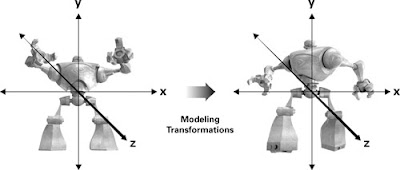
Modeling transfermation: Object Space --> World Space.It makes the model change its shape;
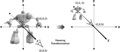 Viewing transfermation: World Space -->Eye Space . It puts eyes at the original.
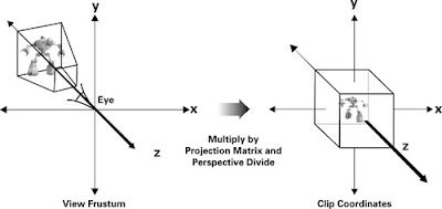
Project transfermation: Eyes Space --> Clip(Project) Space. Changing View frustum to a CUBIC space, in which it is more convenient for clipping.
The Modelview Matrix
Most lighting and other shading computations involve quantities such as positions and surface normals. In general, these computations tend to be more efficient when performed in either eye space or object space. World space is useful in your application for establishing the overall spatial relationships between objects in a scene, but it is not particularly efficient for lighting and other shading computations.
For this reason, we typically combine the two matrices that represent the modeling and view transforms into a single matrix known as the modelview matrix. You can combine the two matrices by simply multiplying the view matrix by the modeling matrix
2. The Transform
Modeling transfermation: Object Space --> World Space.It makes the model change its shape;
Viewing transfermation: World Space -->Eye Space . It puts eyes at the original.Project transfermation: Eyes Space --> Clip(Project) Space. Changing View frustum to a CUBIC space, in which it is more convenient for clipping.
The Modelview Matrix
Most lighting and other shading computations involve quantities such as positions and surface normals. In general, these computations tend to be more efficient when performed in either eye space or object space. World space is useful in your application for establishing the overall spatial relationships between objects in a scene, but it is not particularly efficient for lighting and other shading computations.
For this reason, we typically combine the two matrices that represent the modeling and view transforms into a single matrix known as the modelview matrix. You can combine the two matrices by simply multiplying the view matrix by the modeling matrix
2009-09-03
Computer Graphics Practical.
1. Point
CPoint(n)
2. Mesh
Quad or Triangle construction from Points
3. FillMesh
Using polygon filling algorithm to determine each point in polygon
4. Calculate each point's color with light & texture
For vertexs
Ambient light: Ambient Light Intensity * Ambient Reflection Coefficient * RGB
Diffuse light: Diffuse Light Intensity * Diffuse Reflection Coefficient *cos(θ)* RGB
-->L vector = Light Position - Point ; N vector = Point Normal;
--> cos(θ) = L · N/|L||N|
For other p0ints
Gourand: Each vertex color of the mesh -> BilinearInterpolation ->This Point Color
Phong: Each vertex normal of the mesh -> BilinearInterpolation -> This Point Normal -> Color
CPoint(n)
2. Mesh
Quad or Triangle construction from Points
3. FillMesh
Using polygon filling algorithm to determine each point in polygon
4. Calculate each point's color with light & texture
For vertexs
Ambient light: Ambient Light Intensity * Ambient Reflection Coefficient * RGB
Diffuse light: Diffuse Light Intensity * Diffuse Reflection Coefficient *cos(θ)* RGB
-->L vector = Light Position - Point ; N vector = Point Normal;
--> cos(θ) = L · N/|L||N|
For other p0ints
Gourand: Each vertex color of the mesh -> BilinearInterpolation ->This Point Color
Phong: Each vertex normal of the mesh -> BilinearInterpolation -> This Point Normal -> Color
订阅:
博文 (Atom)